Design and Implementation of a GIS Model for Identifying Isolated Wetlands – Southeast Isolated Wetland Assessment Study Level 1 Assessment
Note: This page describes methods and results of a GIS analysis performed for the Southeast Isolated Wetland Assessment project (SEIWA), summarized here.
Overview
The Southeast Isolated Wetland Assessment project (SEIWA) Level 1 assessment began by using digital elevation models (DEMs) and a GIS “sink” algorithm to create candidate polygon sinks representing low spots in the landscape that could be isolated wetlands. These polygons were then overlaid with existing hydrography, soils, floodplains, wetland, and land cover layers, on infrared imagery, to remove obviously connected features, and then to score the remaining features as to their likelihood to be isolated wetlands. These candidate isolated wetland polygons were then randomly selected for Level 2 assessment.
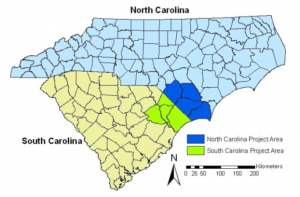
Project study area
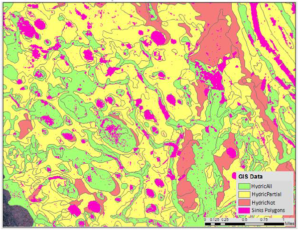
Hydric soils overlapping with elevation derived sink polygons
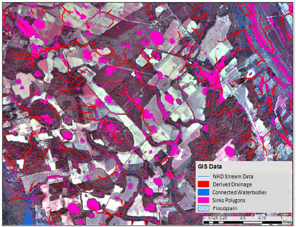
Stream and drainage connectivity with elevation derived sinks
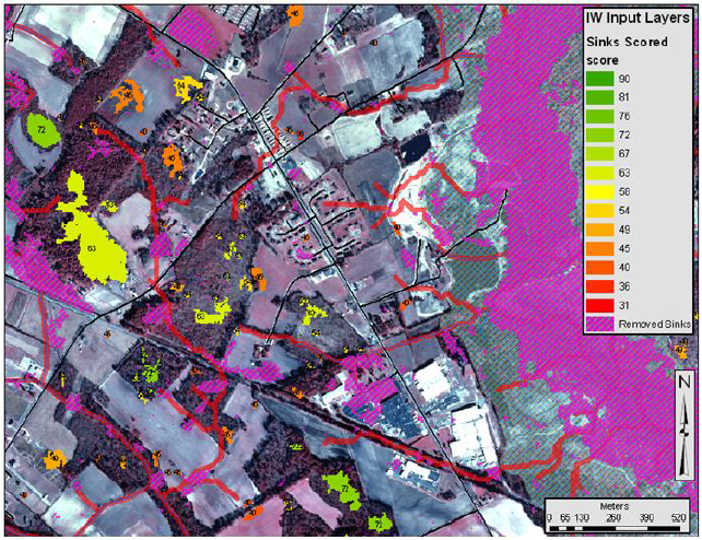
Example area of scored polygons color coded by isolated wetland likelihood
Predictive Mapping Tool Development
A GIS Isolated Wetland Predictive Mapping tool was developed using these steps-
1. Elevation data: A layer of vector polygon sinks was generated from raster elevation data (LiDAR for five counties, USGS hypsography elevation data for three counties). This was derived using a “fill” algorithm in ArcGIS Spatial Analyst.
2. Wetlands: Wetland likelihood was then determined by overlaying GIS layers from wetland soils data, National Wetland Inventory (NWI) data, North Carolina Coastal Region Evaluation of Wetland Significance (NC-CREWS) wetland layer, and feature extraction of “black spots” which are dark areas visible in infrared imagery, often associated with wetland features. Likelihood of ditching connectivity was determined using road layers and agricultural land cover.
3. Connections: Isolated wetlands are not connected by water flow or drainage. Floodplain maps, floodplain soils data, streams, and land cover data were compiled for the study area. A masking procedure was then used to remove polygon sinks that had a low probability of being isolated wetlands. (Assumptions were that floodplains do not contain isolated wetlands, riverine soils occur in floodplains, wetlands intersecting streams do not contain floodplains, and wetlands in agricultural land cover and along roadways are likely to be ditched).
4. Intersections: The aforementioned GIS layers of water and land features were analyzed as to how they intersected with polygon sinks derived from elevation data. The polygons were then each scored from 1 to 10 as to their likelihood of being isolated wetlands, using information from each of the data layers. The result was a subset of polygons described as candidate sinks. The team visited about 40 locations of known isolated wetlands in the eight county study area to help calibrate the model.
Hindcasting wetland loss
The goal of the GIS hindcasting analysis was to map historic isolated wetlands to determine their loss as a result of changes in land cover in the study counties. We compared the extent of Natural Resources Conservation Service (NRCS) hydric soils against more modern wetland coverages (NWI and NC-CREWS) to estimate historic total wetland loss in the study area and (2) used National Land Cover Dataset land cover changes from 1992 to 2001 to estimate the rate of isolated wetland loss in more recent times. Historic wetland loss was estimated by comparing total hydric soils acreage with total wetland acreages assembled from either NC-CREWS wetland coverages or NWI wetland coverages (depending on the county) as estimates of wetland extent in the late 1980s to early 1990s.
Results of Level 1 GIS Analysis
Elevation data source mattered – a LiDAR derived mapping tool produced 322 to > 1,500 candidate sinks per square mile, whereas a hypsography derived mapping tool produced a much smaller 22 to 27 candidate sinks per square mile.
Wetland loss varied by county – Just over 9 percent of wetlands were estimated to have been lost across the study area over 2 decades, with individual counties ranging from zero to 20% total wetland loss and isolated wetlands loss estimated at between 5 percent and 19 percent over a 9 year period (1992-2001) in two counties of interest.